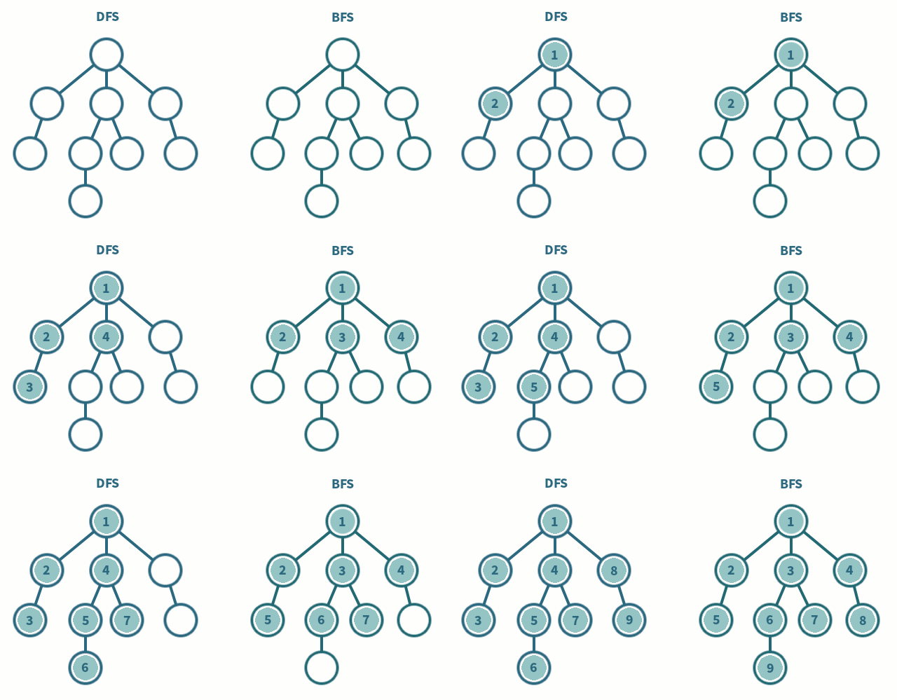
Tree Traversal Space Requirements

TLDR

Tree traversal (or search) comes in two forms, depth first or breadth first. Here is an informal derivation of the space required to traverse trees iteratively using FIFO queues or LIFO stacks. We will end up with two formulas we can use to quite accurately predict how much space is required.

Assumptions

To make things simpler we will only consider "perfect" trees with depth \( D \) and each node having exactly \( \mu \) children if they are not leaf nodes. Only nodes at the final depth/layer are leaf nodes. It is better explained with an example:

After examining the tree long enough we can convince ourselves quite surely that for a tree with \( n \) nodes can be expressed as a sum of the number of nodes at each depth: $$ n = \sum_{d=1}^{D}{\mu^{d-1}} $$

UPDATE: Also we will assume that nodes only have references to their children. This is a very general assumption and as such it serves as a good benchmark for comparing the improvements gained from other algorithms/tree layouts. For instance the example tree shown above would be implemented in C with something like this:

typedef struct node node;
struct node {
    node *left;
    node *right;
}

Breadth first

If we were to visit the nodes breadth first using a FIFO queue, (which the recursive form can also be reduced to), we can easily see that we need to at most store the number of nodes corresponding to the bottom-most layer, \( \mu^{D-1} \), i.e. the number of leaf nodes. So we need to expand the sum to find it in terms of \( n \): $$ n = \frac{\mu^D - 1}{\mu - 1} $$ $$ \mu^{D-1} = n \Big( 1 - \frac{1}{\mu} \Big) + \frac{1}{\mu} $$

Once you look at the asympotic complexity you end up with \( O(n) \) which makes it look really horrible but it is what it is.

Depth first

Deriving the space requirements for depth first traversal using a LIFO stack is a bit more involved. First we consider the tree obtained from \( \mu = 3 \) and \( D = 4 \), truncated for clarity:

If we follow the stack size during the execution of a depth-first traversal, we see something like the following:

The green boxes show the nodes that are about to be traversed, in chunks of \( \mu \) and the red boxes show the waiting nodes in chunks of \( \mu - 1 \). We can now spot a pattern and see that the space required, right before we need to traverse nodes of d^th depth is given by: $$ \text{space}(d) = (\mu - 1)(d - 2) + \mu $$

Let's evaluate it and see that it holds for the stack shown above:

Now just evaluate \( \text{space}(D) \) and expand the terms to obtain a generalised expression for the maximum storage required: $$ D(\mu - 1) - \mu + 2 $$

Again we need play with the terms to obtain something in terms of \( n \). From the previous equations used in the breadth first traversal: $$ n = \frac{\mu^D - 1}{\mu - 1} $$ $$ D = \log_{\mu}{(n(\mu - 1) + 1)} $$ $$ \text{space}(D) = (\mu - 1)\log_{\mu}{(n(\mu - 1) + 1)} - \mu + 2 $$

Now to remove the constant terms and put it in asympotic form: $$ O(\log{n}) $$

Which arguably looks much better than what it actually is. Also note that it is interesting to see that if we have a \( \mu = 2 \), the space requirements are exactly $$ \log_{2}{(n + 1)} = D $$

Justification

To show (rather inelegantly) that the above algorithms and formulas work, you can run the following Python program to prove that the formulas are correct up to certain values, unless you'd want to wait infinitely long:

from collections import deque, namedtuple


Node = namedtuple('Node', ['children'])


def depth_first(node):
    proc = [node]
    while proc:
        yield len(proc)
        node = proc.pop()
        proc.extend(node.children)


def breadth_first(node):
    proc = deque([node])
    while proc:
        yield len(proc)
        node = proc.popleft()
        proc.extend(node.children)


def generate_tree(mu, d):
    root = Node([])
    prev = [root]
    for _ in range(d - 1):
        current = []
        for parent in prev:
            for _ in range(mu):
                child = Node([])
                parent.children.append(child)
                current.append(child)
        prev = current
    return root


def predict_breadth(mu, d):
    return mu ** (d - 1)


def predict_depth(mu, d):
    return d*(mu - 1) - mu + 2


if __name__ == '__main__':
    for mu in range(2, 5):
        for d in range(1, 6):
            t = generate_tree(mu, d)
            depth = max(depth_first(t))
            breadth = max(breadth_first(t))
            print(
                (mu, d),
                depth == predict_depth(mu, d),
                breadth == predict_breadth(mu, d),
            )

You should get the following output when executed:

$ python t.py
(2, 1) True True
(2, 2) True True
(2, 3) True True
(2, 4) True True
(2, 5) True True
(3, 1) True True
(3, 2) True True
(3, 3) True True
(3, 4) True True
(3, 5) True True
(4, 1) True True
(4, 2) True True
(4, 3) True True
(4, 4) True True
(4, 5) True True

Summary

The space requirements for a breadth first traversal of a "perfect" tree with number of children (branching factor) \( \mu \) and depth \( D \) is given by: $$ \mu^{D-1} \approx O(n) $$

And the same for depth first: $$ D(\mu - 1) - \mu + 2 \approx O(\log{n}) $$

These look really horrendous when you plug in values because it's the space required to traverse the whole tree. For searching (DFS or BFS) less than the whole tree would usually need to be traversed.

These are probably of no practical purpose. However one rather odd thing we can do (once we have devised a way to optimally find values of \( \mu \) and \( D \) for "imperfect" trees) is to accurately pre-allocate just enough space for traversal in order to avoid the stacks/queues being resized while the traversal is in progress, which may be something that the real-time folks might be interested in.

Again, these expressions are only for a tree with very general assumptions. Different representations will allow for traversals with different space and time properties, and as pointed out in the discussion on reddit, there are some representations where a search may not require any extra space at all.

A digression: with \( \mu = 1 \) we've essentially made our tree into a list. It's reassuring to see that the formulas work for this case as well, as both algorithms are now the same and consume the same space, 1.