This article documents my rather fruitless quest to model the probability distribution of the number of turns (throws of the dice) required to complete a Snakes and Ladders game, not just for one specific board, but for any board that fits the model. I hope by writing it up, like explaining to someone else I'd get an insight and solve it soon.
For simplicity and generality, the board is modelled using (only[2]) four parameters \( (n, f, p, q) \) where:
Strictly speaking, the last two parameters are not really probabilities in the sense of the word. The probability of a tile being a snake, ladder, or blank is dependent on the type of previous tile that led to the current tile. If it was a snake or a ladder, the next tile would definitely be blank, because the top of a ladder cannot lead to another ladder or snake, and similarly for the tail of a snake. Otherwise:
So the resultant decision tree can be recursively traversed and defined using the following algorithm. For succintness I'll write the code for the case where we model \( (N, 10, 0.1, 0.1) \), but it is easy to generalise for all cases:
def traverse(p, n, prev, N, turns):
    if n >= N:
        yield p, turns
        return
    m = 1.0
    if prev == BLANK:
        m = 1 - q  # 1 - q
        if n > 10:
            m = 0.8  # 1 - p - q
            yield from traverse(0.1*p, n-10, SNAKE, N, turns)
        yield from traverse(0.1*p, n+10, LADDER, N, turns)
    p_dice = 1/6 * p * m
    for i in range(1, 7):
        yield from traverse(p_dice, n+i, BLANK, N, turns+1)
It is important (we will see why later) that the order of iteration is
depth first. Even with the iterative form of the algorithm and the restrictions
we've imposed, it is incredibly difficult to traverse the full tree for
larger values of \( n \) without tacking on yet more restrictions. Part
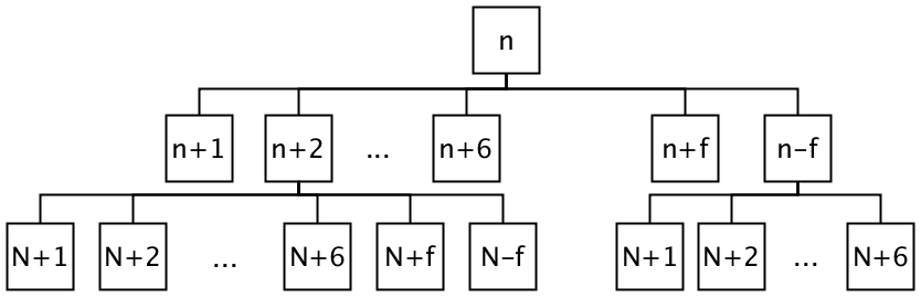
of the tree would look like the following:
Regardless of the type of the algorithm; recursive or iterative, a data-structure is needed to store part of the tree. As Figure 1 shows, even with some pruning of the possibilities, the width of the decision tree grows extremely quickly.
Therefore if we choose breadth first iteration our memory cost would be very large – growing at the rate of at least \( 6^d \), where \( d \) is the current depth of the tree.
However if we only choose to store the nodes depth first, remembering that we don't have to store the full tree, we can bound the memory usage by imposing a hard limit on the depth of the tree[3].
In the program I wrote, such a limit does exist, though admittedly, it is chosen arbitrarily depending on my patience. Even with so many limits imposed, it is still time consuming to find the probability distribution due to the sheer width of the decision tree. The iterative, LIFO stack-based Go version is the following:
import "fmt"

type config struct {
	Snake  float64
	Ladder float64
}

type event struct {
	p         float64
	n         int
	prevBlank bool
	turns     int
	depth     int
}

func pspace(P config, maxTile, maxDepth int) map[int]float64 {
	h := map[int]float64{}
	Q := []event{{1.0, 1, false, 0, 0}}
	var ev event
	for len(Q) > 0 {
		ev, Q = Q[len(Q)-1], Q[:len(Q)-1]
		if ev.n >= maxTile {
			h[ev.turns] += ev.p
			continue
		}
		if ev.depth >= maxDepth {
			h[-1] += ev.p
			continue
		}
		t := ev.depth + 1
		p := 1.0
		if ev.prevBlank {
			p = 1 - P.Ladder
			if ev.n > 10 {
				p = 1 - P.Ladder - P.Snake
				Q = append(Q, event{ev.p * P.Snake, ev.n - 10, false, ev.turns, t})
			}
			Q = append(Q, event{ev.p * P.Ladder, ev.n + 10, false, ev.turns, t})
		}
		pDice := ev.p * p * (1 / 6.0)
		for i := 0; i < 6; i++ {
			Q = append(Q, event{pDice, ev.n + i + 1, true, ev.turns + 1, t})
		}
	}
	return h
}
At this point I've pretty much tried every thing I know that would affect
the running time of the algorithm; for instance I originally wanted to use
the Fraction class in Python to get exact probabilities, now
I'm more than happy if I even get any probabilities. I managed to
extract the following gem, for \( (20, 10, 0.1, 0.1) \) with a maximum
depth of 11.
| \(n\) | \(\Pr[{\text{turns}=n}]\) | cumulative |
|---|---|---|
| \(2\) | \(0.060000000000000026\) | \(0.060000000000000026\) |
| \(3\) | \(0.14207407407407407\) | \(0.2020740740740741\) |
| \(4\) | \(0.1641989197530908\) | \(0.36627299382716494\) |
| \(5\) | \(0.21107717849789398\) | \(0.5773501723250589\) |
| \(6\) | \(0.1755133581316801\) | \(0.752863530456739\) |
| \(7\) | \(0.10296277771903693\) | \(0.855826308175776\) |
| \(8\) | \(0.057477264335094154\) | \(0.9133035725108701\) |
| \(9\) | \(0.031955757099463473\) | \(0.9452593296103337\) |
| \(10\) | \(0.01413115919648122\) | \(0.9593904888068149\) |
| \(11\) | \(0.00012099234715204245\) | \(0.9595114811539669\) |
| \(\infty\) | \(0.040488518840564605\) | \(0.9999999999945315\) |
But I yet to give up all hope! There are still a couple of tricks that I have not used to squeeze out all possible performance. Some possible things I have in mind include:
Taking a cue from the very clever Hashlife algorithm, I should start thinking about hashing the subtrees (and looking into how to do it without exploding in memory usage) to see if I get any performance benefits from not having to re-evaluate the repeated paths.
Maybe memoization or using a dynamic programming method would also help the algorithm perform much better in this case. The exact, final probabilities change each time (which may be non-trivial to manage), but the tree and the possible paths remain the same; pre-computing the trees may help.